In a wide range of motions, the velocity changes from moment to moment. To describe the manner in which it changes, the concept of acceleration is needed. The velocity of a moving object may change in a number of ways. For example, it may increase, as it does when the driver of a car steps on the gas pedal to pass the car ahead. Or it may decrease, as it does when the driver applies the brakes to stop at a red light. In either case, the change in velocity may occur over a short or a long time interval. To describe how the velocity of an object changes during a given time interval, we now introduce the new idea of acceleration.Examples of objects in accelerated motion include automobiles that are speeding up, drivers applying brakes, falling objects, and objects thrown straight upward.

There are several parallels between acceleration and velocity. Both are rates of change: acceleration is the time rate of change of velocity, and velocity is the time rate of change of position. Both acceleration and velocity have average and instantaneous forms. The area under a velocity-time graph is equal to the object’s displacement and that the area under an acceleration-time graph is equal to the object’s velocity.

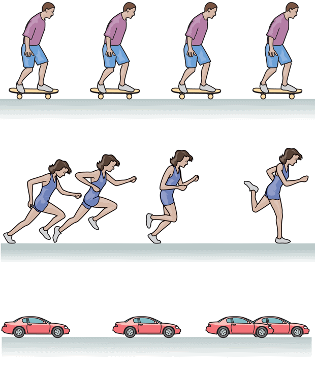
considering a plane during takeoff. Focuses attention on how the plane's velocity changes along the runway. During an elapsed time interval $\Delta t = t_f - t_i$, the velocity changes from an initial value of $\vec{v_i}$ to a final velocity of $\vec{v_f}$. The change $\Delta \vec{v}$ in the plane's velocity is its final velocity minus its initial velocity, so that $\Delta \vec{v} = \vec{v_f} - \vec{v_i}$ The average acceleration a is defined in the following manner, to provide a measure of how much the velocity changes per unit of elapsed time.

$$\text{Average acceleration}= \dfrac{\text{Change in velocity}}{\text{Elapsed time}}$$

$$\bar {\vec{a}}= \dfrac{\vec{v_f} - \vec{v_i}}{t_f - t_i}=\dfrac{\Delta \vec{v}}{\Delta t}$$

SI Unit of Average Acceleration: meter per second squared ($\mathrm{m/s^2}$ )

We saw that velocity is a vector (it has magnitude and direction), so acceleration is a vector too points in the same direction as $\Delta \vec{v}$, the change in the velocity. But for one dimensional motion, we will follow the usual custom, we need only use a plus or minus sign to indicate acceleration direction relative to a chosen coordinate axis. (Usually, right is + left is -)

hints

• The word deceleration has the common popular connotation of slowing down. We will not use this word because it confuses the definition we have given for negative acceleration.
• Whenever the acceleration and velocity vectors have opposite directions, the object slows down and is said to be "decelerating."
• Negative acceleration does not necessarily mean that an object is slowing down. If the acceleration is negative and the velocity is negative, the object is speeding up.
• Acceleration is caused by force, force and acceleration are both vectors, and the vectors are in the same direction. it is easier to think about what effect a force will have on an object than to think only in terms of the direction of the acceleration.

The instantaneous acceleration, $\vec{a}$, can be defined in analogy to instantaneous velocity as the average acceleration over an infinitesimally short time interval at a given instant:

$$\vec{a} = \lim_{\Delta t \to 0} \dfrac{\Delta \vec{v}}{\Delta t}$$

Here $\Delta \vec{v}$ is the very small change in velocity during the very short time interval $\Delta t$.

(approaching zero in the limit), the average acceleration and the instantaneous acceleration become equal. Moreover, in many situations the acceleration is constant, so the acceleration has the same value at any instant of time.

hints

• In the future, we will use the word acceleration to mean "instantaneous acceleration."
• In one-dimensional motion, the acceleration of a particle equals the second derivative of the particle’s position x with respect to time: $$\vec{a_x} = \dfrac{d \vec{v_x}}{d t}= \dfrac{d}{d t} \left( \dfrac{d \vec{x}}{d t} \right)= \dfrac{d^2 \vec{x}}{d t^2}$$

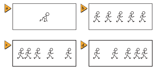
Consider the following motion diagrams, How would you describe the motion of the person in each case?

The most important thing to notice in these motion diagrams is the distance between successive positions.

• a. the person is motionless.
• b. she is moving at a constant speed
• c. she is speeding up
• d. she is slowing down

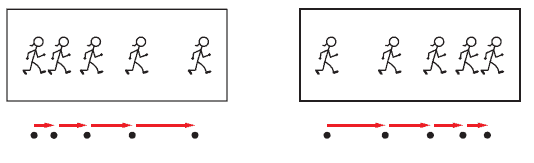
What does a particle-model motion diagram look like for an object with changing velocity? the following image shows the particle-model motion diagrams below the motion diagrams of a jogger speeding up and slowing down:

For a motion diagram to give a full picture of an object’s movement, it also should contain information about acceleration. This can be done by including average acceleration vectors. These vectors will indicate how the velocity is changing. There are two major indicators of the change in velocity in this form of motion diagram. The change in the spacing of the dots and the differences in the lengths of the velocity vectors indicate the changes in velocity. If an object speeds up, each subsequent velocity vector is longer. If the object slows down, each vector is shorter than the previous one.

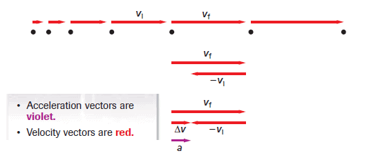
To determine the length and direction of an average acceleration vector, subtract two consecutive velocity vectors, as shown in the following motion diagram whitch shows an object moving in the positive direction and speeding up:

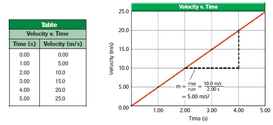
Just as it was useful to graph a changing position versus time, it also is useful to plot an object’s velocity versus time, which is called a velocity-time, or v-t graph. For example, the following Table shows the data for a car that starts at rest and speeds up along a straight stretch of road:

Notice that this graph is a straight line, which means that the car was speeding up at a constant rate. The rate at which the car’s velocity is changing can be found by calculating the slope of the velocity-time graph. The rate at which an object’s velocity changes is called the acceleration of the object. When the velocity of an object changes at a constant rate, it has a constant acceleration.

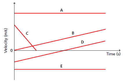
For example, Graphs A, B, C, D, and E in the following Figure represent the motions of five different runners:

• A. The slopes of Graph A is zero. Thus, the acceleration is zero (constant velocity to the positive direction).
• B. The slopes of Graph B indicates a constant, positive acceleration (the speed increased because it shows positive velocity and acceleration).
• C. Graph C has a negative slope. This means that the acceleration and velocity are in opposite directions. (Graph C shows motion that begins with a positive velocity, slows down, and then stops.The point at which Graphs C and B cross shows that the runners’ velocities are equal at that point. It does not, however, give any information about the runners’ positions.).
• D. The slope of Graph D is positive. Because the velocity and acceleration are in opposite directions, the speed decreases and equals zero at the time the graph crosses the axis. After that time, the velocity and acceleration are in the same direction and the speed increases (Graph D indicates movement that starts out toward the negative direction, slows down, and for an instant gets to zero velocity, and then moves to the positive direction with increasing speed).
• E. The slopes of Graph E is zero. Thus, the acceleration is zero (constant velocity to the negative direction).

 

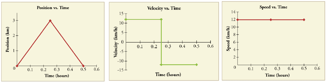
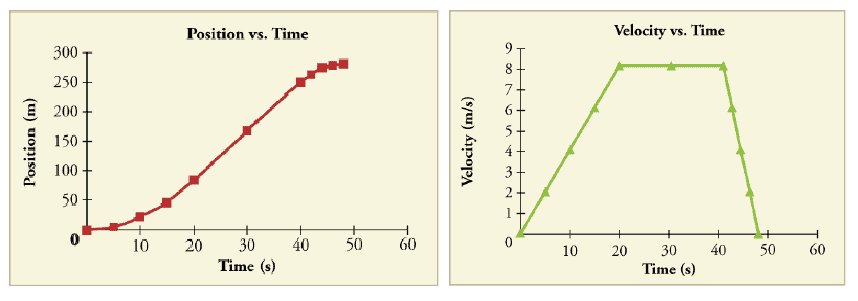
Here is some examples of the graphical analysis of velocity:

If the acceleration of a particle varies in time, its motion can be complex and difficult to analyze. A very common and simple type of one-dimensional motion (in a straight line), however, is that in which the acceleration is constant. In this case, the instantaneous and average accelerations are equal, and the velocity changes at the same rate throughout the motion. This situation occurs often enough that we identify it as an analysis model. In the discussion that follows, we generate several equations that describe the motion of a particle for this model.These equations entail no new concepts, because they will be obtained by combining the familiar ideas of displacement, velocity, and acceleration. However, they will provide a very convenient way to determine certain aspects of the motion, such as the final position and velocity of a moving object.

Notation in physics varies from book to book; and different instructors use different notation, to simplify it a bit for our discussion here of motion at constant acceleration we assume that the object is located at the origin ($\vec{x_i}=0, t_i=0$). Furthermore, in the equations that follow, as is customary, we dispense with the use of boldface symbols overdrawn with small arrows for the displacement, velocity, and acceleration vectors. We will, however, continue to convey the directions of these vectors with plus or minus signs.

With this assumption, the displacement ($\vec{\Delta x}=\vec{x_f} - \vec{x_i}$) becomes $\vec{\Delta x}=x$, the elapsed time ($\Delta t=t_f - t_i$) becomes $\Delta t=t$, and the average velocity during the time interval $t$ will be $\bar{v}=\dfrac{\vec{\Delta x}}{\Delta t}= \dfrac{x}{t}$. The displacement $x$ at time $t$ can be obtained from the average velocity:

$$x=\bar{v} t$$

Because the acceleration is constant, the velocity increases at a constant rate. Thus, the average velocity in any time interval can be obtained as the arithmetic mean of the initial velocity and the final velocity $\left( \bar{v}=\frac{1}{2} (v_f + v_i) \right)$, this equation applies only if the acceleration is constant and cannot be used when the acceleration is changing. The displacement at time $t$ can now be determined as:

$$x= \frac{1}{2} (v_f + v_i) t \;\;\;\;\;\;\;\; \rightarrow \;\; \textbf{(1)}$$

For a complete description of the motion, it is also necessary to know the final velocity and displacement at time $t$. The final velocity $v_f$ can be obtained directly from the constant acceleration equation $\left( \bar{a}=a=\dfrac{v_f - v_i}{t} \right)$, or:

$$v_f= v_i + at \;\;\;\;\;\;\;\; \rightarrow \;\; \textbf{(2)}$$

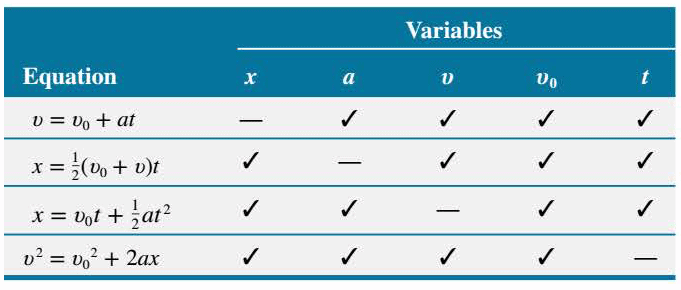
Notice in Equations (1) and (2) that there are five kinematic variables:

• $x$ = displacement
• $a$ = acceleration (constant)
• $v_f$ = final velocity at time $t$
• $v_i$ = initial velocity at time $0 s$
• $t$ = time elapsed since $0 s$

Each of the two equations contains four of these variables, so if three of them are known, the fourth variable can always be found.

Algebraically combining the two equations into a single equation and eliminating the final velocity, we find that the displacement $x$ is:

$$x= v_i t + \frac{1}{2} a t^2 \;\;\;\;\;\;\;\; \rightarrow \;\; \textbf{(3)}$$

The first term ($v_i t$) on the right side of this equation represents the displacement that would result if the acceleration were zero and the velocity remained constant at its initial value of $v_i$. The second term $\left( \frac{1}{2} a t^2 \right)$ gives the additional displacement that arises because the velocity changes ($a$ is not zero) to values that are different from its initial value.

Even if the time interval is not given, we can still calculate the displacement. We can solve Equation (2) for the time $t$, and then make this substitution into Equation (3). The result is $\left( x= \dfrac{(v_f^2 -v_i^2)}{2a} \right)$. Solving for $v_f^2$ gives:

$$v_f^2= v_i^2 + 2ax \;\;\;\;\;\;\;\; \rightarrow \;\; \textbf{(4)}$$

The following table presents a summary of the equations that we have been considering. These equations apply when an object moves with a constant acceleration along a straight line. Assuming that $x_i = 0 m$ at $t_i = 0 s$, each equation contains four of the five kinematic variables, as indicated by the check marks in the table:

Everyone has observed the effect of gravity as it causes objects to fall downward. In the absence of air resistance, it is found that all bodies at the same location above the earth fall vertically with the same acceleration. Furthermore, if the distance of the fall is small compared to the radius of the earth, the acceleration remains essentially constant throughoult the descent. This idealized motion, in which air resistance is neglected and the acceleration is nearly constant, is known as free-fall. Since the acceleration is constant in free-fall, the equations of kinematics can be used.

The acceleration of a freely falling body is called the acceleration due to gravity, and its magnitude (without any algebraic sign) is denoted by the symbol $g$. The acceleration due to gravity is directed downward, toward the center of the earth. Near the earth's surface, $g$ is approximately $9.8 \;\mathrm{m/s^2}$. A nice demonstration of free-fall was performed on the moon by astronaut David Scott, who dropped a hammer and a feather simultaneously from the same height. Both experienced the same acceleration due to lunar gravity and consequently hit the ground at the same time. The acceleration due to gravity near the surface of the moon is approximately one-sixth as large as that on the earth.

When the equations of kinematics are applied to free-fall motion, it is natural to use the symbol $y$ for the displacement, since the motion occurs in the vertical or $y$ direction.

The acceleration due to gravity is always a downward-pointing vector. It describes how the speed increases for an object that is falling freely downward. This same acceleration also describes how the speed decreases for an object moving upward under the influence of gravity alone, in which case the object eventually comes to a momentary halt and then falls back to earth.

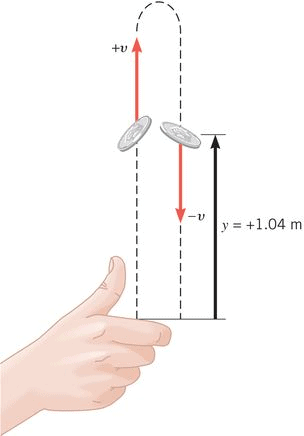
The motion of an object that is thrown upward and eventually returns to earth has a symmetry that is useful to keep in mind from the point of view of problem solving. The calculations just completed indicate that a time symmetry exists in free-fall motion, in the sense that the time required for the object to reach maximum height equals the time for it to return to its starting point. A type of symmetry involving the speed also exists, for a given displacement along the motional path, the upward speed of the object is equal to its downward speed, but the two velocities point in opposite directions. This symmetry involving the speed arises because the object loses 9.8 m/s in speed each second on the way up and gains back the same amount each second on the way down.